Freeze Multiple Columns In Excel For Mac
When working with large Excel spreadsheets, the column and row headings located at the top and down the left side of the worksheet disappear if you scroll too far to the right or too far down. To avoid this problem, freeze the rows and columns. Freezing locks specific columns or rows in place so that no matter where you scroll they're always visible on the top or side of the sheet.
Freeze panes to lock the first row or column. Excel for Office 365 for Mac Excel 2019 for Mac Excel 2016. Top row and the first column. To freeze multiple.
Challenger comic viewer for windows. Instructions in this article apply to Excel 2019, 2016, 2013, 2010, 2007; Excel Online, and Excel for Mac.
Freeze the Top Row of a Worksheet
Freezing the top row of a worksheet is a great way to keep your Excel headings visible at all times. Follow these three easy steps to get that header to stay in place.
To freeze the top row of a worksheet:
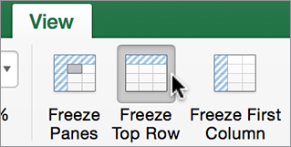
Select View on the ribbon.
Select Freeze Panes. If you're using Excel for Mac, skip this step.
Select Freeze Top Row.
A border appears just below Row 1 to indicate that the area above the line has been frozen. The data in row 1 remains visible as you scroll down because the entire row is pinned to the top of Excel.
Freeze the First Column of a Worksheet
Quicken for mac 2017 why dont all future transaction appear in accounts. In addition to freezing the first row of a worksheet, you can also freeze the first column just as easily.

To freeze the first column of a worksheet:
Select View.
Select Freeze Panes. If you're using Excel for Mac, skip this step.
Select Freeze First Column.
The entire column A area is frozen, indicated by the black border between column A and B. Enter some data into column A, scroll to the right, and you'll see the data move with you.
Freeze Both Columns and Rows of a Worksheet
You can also freeze all the rows above the active cell and all the columns to the left of the active cell. These columns and rows remain on the screen at all times, no matter how far you scroll.
To keep specified rows and columns visible:
Select a cell that is below the row that you want frozen and to the right of the column you want frozen. These are the rows and columns that stay visible when you scroll.
Select View.
Select Freeze Panes. If you're using Excel for Mac, skip this step.
Select Freeze Panes.
Two black lines appear on the sheet to show which panes are frozen. The rows above the horizontal line are kept visible while scrolling. The columns to the left of the vertical line are kept visible while scrolling.
Unfreeze Columns and Rows in Excel
When you no longer want certain rows and columns to stay in place when you scroll, unfreeze all the panes in Excel. The data in the frames will remain, but the rows and columns that were frozen will return to their original positions.
To unfreeze panes, select View > Freeze Panes > Unfreeze Panes. Except on Excel for Mac, where you select View > Unfreeze Panes instead.