Unable To Change Date Format In Excel For Mac

Jun 27, 2017 - If you attempt to change the format of a cell containing a 'date', and the display does not change, then the cell contains Text rather than a true.

The first part of our tutorial focuses of formatting dates in Excel and explains how to set the default date and time formats, how to change date format in Excel, how to create custom date formatting, and convert your dates to another locale. Along with numbers, dates and times are the most common data types people use in Excel. However, they may be quite confusing to work with, firstly, because the same date can be displayed in Excel in a variety of ways, and secondly, because Excel always internally stores dates in the same format regardless of how you have formatted a date in a given cell.

Knowing the Excel date formats a little in depth can help you save a ton of your time. And this is exactly the aim of our comprehensive tutorial to working with dates in Excel.

In the first part, we will be focusing on the following features:. Excel date format Before you can take advantage of powerful Excel date features, you have to understand how Microsoft Excel stores dates and times, because this is the main source of confusion. While you would expect Excel to remember the day, month and the year for a date, that's not how it works. Excel stores dates as sequential numbers and it is only a cell's formatting that causes a number to be displayed as a date, time, or date and time. Dates in Excel All dates are stored as integers representing the number of days since January 1, 1900, which is stored as number 1, to December 31, 9999 stored as 2958465.

In this system:. 2 is 2-Jan-1900. 3 is 3-Jan-1900. 42005 is 1-Jan-2015 (because it is 42,005 days after January 1, 1900) Time in Excel Times are stored in Excel as decimals, between.0 and.99999, that represent a proportion of the day where.0 is 00:00:00 and.99999 is 23:59:59. For example:. 0.25 is 06:00 AM.

0.5 is 12:00 PM. 0.541655093 is 12:59:59 PM Dates & Times in Excel Excel stores dates and times as decimal numbers comprised of an integer representing the date and a decimal portion representing the time. For example:. 1.25 is January 1, 1900 6:00 AM. 42005.5 is January 1, 2015 12:00 PM How to convert date to number in Excel If you want to know what serial number represents a certain date or time displayed in a cell, you can do this in two ways. Format Cells dialog Select the cell with a date in Excel, press Ctrl+1 to open the Format Cells window and switch to the General tab. If you just want to know the serial number behind the date, without actually converting date to number, write down the number you see under Sample and click Cancel to close the window.

If you want to replace the date with the number in a cell, click OK. Excel DATEVALUE and TIMEVALUE functions Use the DATEVALUE function to convert an Excel date to a serial number, for example =DATEVALUE('1/1/2015'). Use the TIMEVALUE function to get the decimal number representing the time, for example =TIMEVALUE('6:30 AM'). To know both, date and time, concatenate these two functions in the following way: =DATEVALUE('1/1/2015') & TIMEVALUE('6:00 AM'). Since Excel's serial numbers begins on January 1, 1900 and negative numbers aren't recognized, dates prior to the year 1900 are not supported in Excel.

If you enter such a date in a sheet, say, it will be a text value rather than a date, meaning that you cannot perform usual date arithmetic on early dates. To make sure, you can type the formula =DATEVALUE(') in some cell, and you will get an anticipated result - the #VALUE!

If you are dealing with date and time values and you'd like to convert time to decimal number, please check out the formulas described in this tutorial:. Default date format in Excel When you work with dates in Excel, the short and long date formats are retrieved from your Windows Regional settings. These default formats are marked with an asterisk (.) in the Format Cell dialog window: The default date and time formats in the Format Cell box change as soon as you change the date and time settings in Control Panel, which leads us right to the next section. How to change the default date and time formats in Excel If you want to set a different default date and/or time formats on your computer, for example change the USA date format to the UK style, go to Control panel and click Region and Language.

If in your Control panel opens in Category view, then click Clock, Language, and Region Region and Language Change the date, time, or number format. On the Formats tab, choose the region under Format, and then set the date and time formatting by clicking on an arrow next to the format you want to change and selecting the desired one from the drop-down list. If you are not sure what different codes (such as mmm, ddd, yyy) mean, click the ' What does the notation mean' link under the Date and time formats section, or check the in this tutorial.

If you are not happy with any time and date format available on the Formats tab, click the Additional settings button in the lower right-hand side of the Region and Language dialog window. This will open the Customize dialog, where you switch to the Date tab and enter a custom short or/and long date format in the corresponding box.

How to quickly apply default date and time formatting in Excel Microsoft Excel has two default formats for dates and time - short and long, as explained in. To quickly change date format in Excel to the default formatting, do the following:. Select the dates you want to format.

On the Home tab, in the Number group, click the little arrow next to the Number Format box, and select the desired format - short date, long date or time. If you want more date formatting options, either select More Number Formats from the drop-down list or click the Dialog Box Launcher next to Number. This will open a familiar Format Cells dialog and you can there. If you want to quickly set date format in Excel to dd-mmm-yy, press Ctrl+Shift+#. Just keep in mind that this shortcut always applies the dd-mmm-yy format, like 01-Jan-15, regardless of your Windows Region settings.

How to change date format in Excel In Microsoft Excel, dates can be displayed in a variety of ways. When it comes to changing date format of a given cell or range of cells, the easiest way is to open the Format Cells dialog and choose one of the predefined formats.

Select the dates whose format your want to change, or empty cells where you want to insert dates. Press Ctrl+1 to open the Format Cells dialog. Alternatively, you can right click the selected cells and choose Format Cells from the context menu. In the Format Cells window, switch to the Number tab, and select Date in the Category list. Under Type, pick a desired date format. Once you do this, the Sample box will display the format preview with the first date in your selected data. If you are happy for the preview, click the OK button to save the format change and close the window.

If the date format is not changing in your Excel sheet, most likely your dates are formatted as text and you have to convert them to the date format first. How to convert date format to another locale Once you've got a file full of foreign dates and you would most likely want to change them to the date format used in your part of the world.

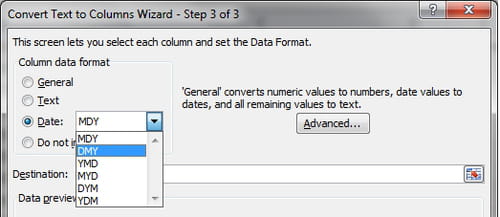
Let's say, you want to convert an American date format (month/day/year) to a European style format (day/month/year). The easiest way to change date format in Excel based on how another language displays dates is as follows:. Select the column of dates you want to convert to another locale.

Press Ctrl+1 to open the Format Cells. Select the language you want under Locale (location) and click OK to save the change. If you want the dates to be displayed in another language, then you will have to create a. Creating a custom date format in Excel If none of the predefined Excel date formats is suitable for you, you are free to create your own.

In an Excel sheet, select the cells you want to format. Press Ctrl+1 to open the Format Cells dialog. On the Number tab, select Custom from the Category list and type the date format you want in the Type box. The easiest way to set a custom date format in Excel is to start from an existing format close to what you want. To do this, click Date in the Category list first, and select one of existing formats under Type.

After that click Custom and make changes to the format displayed in the Type box. When setting up a custom date format in Excel, you can use the following codes. Code Description Example (January 1, 2005) m Month number without a leading zero 1 mm Month number with a leading zero 01 mmm Month name, short form Jan mmmm Month name, full form January mmmmm Month as the first letter J (stands for January, June and July) d Day number without a leading zero 1 dd Day number with a leading zero 01 ddd Day of the week, short form Mon dddd Day of the week, full form Monday yy Year (last 2 digits) 05 yyyy Year (4 digits) 2005 When setting up a custom time format in Excel, you can use the following codes.

Code Description Displays as h Hours without a leading zero 0-23 hh Hours with a leading zero 00-23 m Minutes without a leading zero 0-59 mm Minutes with a leading zero 00-59 s Seconds without a leading zero 0-59 ss Seconds with a leading zero 00-59 AM/PM Periods of the day (if omitted, 24-hour time format is used) AM or PM. If you're setting up a custom format that includes date and time values and you use ' m' immediately after ' hh' or ' h' or immediately before 'ss' or 's', Microsoft Excel will display minutes instead of the month.

When creating a custom date format in Excel, you can use a comma (,) dash (-), slash (/), colon (:) and other characters. For example, the same date and time, say January 13, 2015 13:03, can be displayed in a various ways: Format Displays as dd-mmm-yy 13-Jan-15 mm/dd/yyyy m/dd/yy 1/13/15 dddd, m/d/yy h:mm AM/PM Tuesday, 1/13/15 1:03 PM ddd, mmmm dd, yyyy hh:mm:ss Tue, January 13, 2015 13:03:00 How to create a custom Excel date format for another locale If you want to display dates in another language, you have to create a custom format and prefix a date with a corresponding locale code. The locale code should be enclosed in square brackets and preceded with the dollar sign ($) and a dash (-). Here are a few examples:.

$-409 - English, Untitled States. $-1009 - English, Canada. $-407 - German, Germany. $-807 - German, Switzerland. $-804 - Bengali, India. $-804 - Chinese, China. $-404 - Chinese, Taiwan You can find the full list of locale codes on.

For example, this is how you set up a custom Excel date format for the Chinese locale in the year-month-day (day of the week) time format: The following image shows a few examples of the same date formatted with different locale codes in the way traditional for the corresponding languages: Excel date format not working - fixes and solutions Usually, Microsoft Excel understands dates very well and you are unlikely to hit any roadblock when working with them. If you happen to have an Excel date format problem, please check out the following troubleshooting tips. A cell is not wide enough to fit an entire date If you see a number of pound signs (#####) instead of dates in your Excel worksheet, most likely your cells are not wide enough to fit the whole dates. Double-click the right border of the column to resize it to auto fit the dates. Alternatively, you can drag the right border to set the column width you want. Negative numbers are formatted as dates In all modern versions of Excel 2013, 2010 and 2007, hash marks (#####) are also displayed when a cell formatted as a date or time contains a negative value. Usually it's a result returned by some formula, but it may also happen when you type a negative value into a cell and then format that cell as a date.

If you want to display negative numbers as negative dates, two options are available to you: Solution 1. Switch to the 1904 date system. Go to File Options Advanced, scroll down to the When calculating this workbook section, select the Use 1904 date system check box, and click OK. In this system, 0 is 1-Jan-1904; 1 is 2-Jan-1904; and -1 is displayed as a negative date -2-Jan-1904.

Of course, such representation is very unusual and takes time to get used to, but this is the right way to go if you want to perform calculations with early dates. Use the Excel TEXT function.

Another possible way to display negative numbers as negative dates in Excel is using the TEXT function. For example, if you are subtracting C1 from B1 and a value in C1 is greater than in B1, you can use the following formula to output the result in the date format: =TEXT(ABS(B1-C1),'-d-mmm-yyyy') You may want to change the cell alignment to right justified, and naturally, you can use any other in the TEXT formula.

Unlike the previous solution, the TEXT function returns a text value, that is why you won't be able to use the result in other calculations. Dates are imported to Excel as text values When you are importing data to Excel from a.csv file or some other external database, dates are often imported as text values. They may look like normal dates to you, but Excel perceives them as text and treats accordingly. You can convert 'text dates' to the date format using Excel's DATEVALUE function or Text to Columns feature.

Please see the following article for full details:. This is how you format dates in Excel. In the next part of our guide, we will discuss various ways of how you can insert dates and times in your Excel worksheets. Thank you for reading and see you next week! You may also be interested in:. Hello, Marianne: Hello: I think the easiest way to is to select the cells and use the Text-to-Columns tool in the data tab.

It goes like this: Practice with one cell. My passport for mac help. Select the cell that holds the 'November, 2016'. Choose the Text-to-Columns tool. Choose the Delimited button, click next. Choose the Other button and enter ',' in the field, click next. Then you'll see how Excel will separate the data, click finish. You can select a destination cell if you need to.

Keep in mind that the cell you select will be the first cell of two cells for the separated data. After this you will have the year separated in a destination cell as Date. Go through this same procedure for as many of the cells at one time as you want - one more or one hundred more. Shyam Lal: The easiest way to do this is to Find and Replace the '.' After you've done this Excel will recognize the entries as dates and then you can format them to be displayed in the format that suits you. Here's the procedure: Select the cells that hold the dates you want to change.

Then click the Find and Select tool, then Replace to open the Find and Replace dialogue window Then enter a '.' In the Find What field and a '/' in the Replace With field The first time you do this you should click the Find Next button then the Replace button. This way you can see what the Find and Replace procedure is doing to your data. When you're satisfied that Find and Replace is doing what you want you can click the Replace All button. When this procedure id finished, you can select the newly modified cells and click the Format Cells option and format the entries to be display in the manner you like. Kate: If I understand your question you're asking how to remove two characters from the text string. I would remove them by using the SUBSTITUTE function with a nested SUBSTUTUTE formula like this: =SUBSTITUTE(SUBSTITUTE(K17,'T','),'Z', ') Where the problem string is in K17 this says to Excel substitute nothing for the 'T' and nothing for the 'Z'.

Now, you'll need to copy this down the column and it is only looking for 'T' and 'Z', but if your data has only a 'T' and a 'Z' to remove, this won't take a minute to copy down the column. You can of course substitute another letter or letters for the 'T' and/or 'Z' or something else for the 'nothing'. Hi I have to capture a lot of till slips for an account recon.

I would like to enter, for example 2506 and get out or 25 Jun for example. I cannot seem to find how to do that. I tried following your examples using the RIGHT, MID and LEFT values but it wouldn't accept it even if i used it exactly as shown. I'm at a bit of a loss. Nothing on my format options works as the system is reading the input of 250618 or 2506 as a code for a particular date. Entering each slip date exactly as a date format will be tremendously laborious.

I use the 'CTRL;' to quickly enter the current date and hit 'SPACE' and continue to enter text to provide updates for that date in the same cell. The problem I am having is that regardless of the regional settings for the short date format (in my case 14-Mar-12), it will always use 'dd-mm-yyyy' (i.e. The default date type '.' ) the format I want is 'dd-mmm-yy'. Is there a way to change the default date type format? If I don't enter any text after and exit the cell it will change the format to the desired one. If you enter any text after it will not change it and it will keep it as dd-mm-yyyy (i.e.

Putting the date in a separate cell is not an option.

I'm trying to make the following code for mac, but it doesn't works(in windows this code works fine). I'm originally programming this code in windows, for windows users, but now we have a new co-worker with mac, and that code is the only one with issues. Hopes somebody could help me with this, I don't use mac and don't know why this happens.

So there seems no way with WD tools to test an exFAT formatted drive. DiskWarrior recognizes the drive and identifies the format, but only works on HFS. Does mac support exfat. Does anyone know a way to do a full check of a exFAT formatted drive on a Mac?

Private Sub DateBoxChange Cells(6, 3).Value = Format$(DateBox.Value, 'dd/mmm/yyyy') End Sub The excel version of the mac is: Excel for MAC 2011 14.1.0, and the problem happens when the user input just one number in the textbox.